Phased Array Adjustment for Ham
Radio
Grant Bingeman, P.E.
KM5KG
Introduction
This article presents a lumped-parameter tee-network model of the coupling
between radiating elements in a phased array in order to provide a physical and
intuitive understanding of phased array operation and adjustment interactions.
It then analyzes the performance of a practical phased array antenna which
appeared in a QST magazine construction article.1 The technique of
connecting mismatched feeders to the driven elements in a phased array is an
expedient method for obtaining relative current phases in the elements that
approximate the desired currents. A simple technique to provide instant pattern
adjustability with a variable capacitor is discussed later in the article. This
practical technique helps to compensate for the coarse method of using
mismatched transmission lines to provide phasing.
Basic Theory
A phased array is an antenna having more than one driven element. The desired
radiation pattern is obtained by adjusting the current magnitude and phase in
each element. Ideally, we want to be able to independently adjust the
current magnitude and phase in each element and also obtain a perfect impedance
match to the transmission lines carrying power to each element. It is nearly
impossible to do this by simply fanning out different length transmission lines
from the common feed point to the driven elements. However, a compromise can be
reached, which is the main thrust of this article.
An antenna design is begun by defining a set of desired performance features.
This set may include gain, beamwidth, departure angle, polarization,
front-to-back ratio, front-to-side ratio, impedance and pattern bandwidths,
component stress (current, voltage, compression, tension, shear), overall size
and weight, feed-point impedance, etc. Since many of the desired features
interact and some may be improved only at the expense of others, priorities must
also be assigned to these performance criteria. In other words you must weight
your criteria, and set upper and lower boundaries. Like most things in life,
antenna design is a set of compromises.
In order to efficiently optimize your design, it certainly helps to
understand how the antenna performance features interact on both the
quantitative and qualitative levels. For example, it is generally true that
there is a trade-off between gain and bandwidth. Sometimes a slight improvement
in gain is paid for by a major degradation in bandwidth. Therefore you have to
find a balance, and this depends on the relative importance of each of the
antenna's performance criteria. Obviously if we are operating CW at a single
frequency, we don't care too much about bandwidth. If we are only operating in
the SSB portion of the 20 meter band, then we only care about antenna
performance in the upper half of the band. And so on.
Optimizing algorithms have been around for a long time, and can readily be
applied to antenna design problems. A formula is written to create an error sum
based on each of the weighted antenna performance criteria. Various parameters
in the antenna are adjusted until a minimum error is found. This iterative
process is both an art and a science, and has a jargon all its own. There are
brute-force methods that may take a long time and never reach the best solution,
and there are "intelligent" algorithms that employ advanced mathematical
concepts, and converge quickly. Digital computers love these kinds of tasks.
Since the outcome of such optimization is dependent on the number of
parameters that can be varied, the more the better (usually). Too many knobs can
get a human operator into deep water, whereas a computer program seldom
complains about these iterative exercises. Typical high-gain amateur radio
antennas consist of one driven element and many parasitic elements. The input
parameters to your typical parasitic antenna design would therefore include
element length, diameter and spacing, height above ground, and perhaps some
transmission lines and other discrete components. If you also introduce multiple
RF sources, such that both the source current magnitudes and phases are added to
the adjustable parameter list, then you increase the possibility of finding a
better compromise between all the desired performance features. In other words,
for a given field intensity maybe you can get twice the bandwidth from an array
of two driven elements compared to an array of one driven and one parasitic
element. Or perhaps you can get a certain gain from a driven array that requires
only half the volume of a conventional parasitic array with the same gain.
And so this article will explore the physical inter-actions and
rules-of-thumb that apply when you are designing an antenna having more than one
driven element. Admittedly the complexity of the problem increases exponentially
as we add more knobs to the "box," but a human operator will eventually develop
a feel for the problem by simply turning the cranks and observing what happens.
Since the 1960's, the "box" has often consisted simply of a method-of-moments
antenna analysis program. Some general rules will appear as you play with the
box, and if you read this article carefully, you will find some useful
short-cuts to the antenna design process. Rule number one: write everything down
in a notebook so you don't end up repeating yourself, and enter enough detail so
you can readily verify your results later. Define a simple set of goals and try
to stick by them.
A Starting Point
The behavior of a single isolated antenna element, such as a dipole in free
space, is a simplified or reduced model of an actual antenna. In reality the
behavior of a dipole is influenced by the presence of the earth, weather,
support structures, transmission line, insulators, etc. Often these influences
are minor, but when an additional radiating element is deliberately added to an
antenna, major changes occur in the first element. When both elements are
physically aligned and within a wavelength or so of each other, they are said to
be strongly coupled.
We can loosely tie everything together by observing the current in the
antenna elements, and remembering Ohm's Law. The electric field intensity
produced by an antenna is directly proportional to the currents in that antenna.
For a given power input to an antenna, high-gain multi-element wire antennas
have relatively high currents compared to single-element antennas of comparable
dimensions. This higher gain is manifested as a decrease in the input resistance
to the antenna. For example, assume you have a 144 MHz half-wave dipole fed at
its center. You measure the input impedance and find it to be about 70 + j0
ohms. Then you add a second antenna element consisting simply of a
half-wavelength of wire in parallel with your driven element. As you move this
wire closer to your dipole, you will see the input resistance to the dipole
drop. For a spacing of 30 cm, the input impedance becomes about 25 + j25 ohms
and the field intensity increases by about 3.6 dB in one direction compared to
the dipole alone, and decreases in the opposite direction. The parasitic wire
acts as a reflector at this spacing, but at a much closer spacing it can act as
a director and produce even more gain, albeit in the opposite direction. For a
spacing of 10 cm, the input impedance is about 4 - j20 ohms, and the gain is
about 4.0 dB. However, since the currents are much higher and the input
resistance much lower for this close spacing, you can lose quite a bit of your
input power in the form of i2R losses, depending on the resistance of
the wires. I assumed copper for the gain figures cited; aluminum would yield a
gain of perhaps 3.9 dB, and steel would just about eat up all of our gain for
the 10 cm spacing.
You must never assume that maximum current means maximum gain. If we were to
narrow the spacing between the two antenna elements such that the second element
shorted out the driven element, then the input resistance would approach zero,
the current would get very high, but the field would approach a theoretical
minimum. And remember that real wires and real insulators have losses, and the
higher the currents in these wires, and the higher the voltages across these
insulators, the more RF power will be lost as heat. Or worse, you may encounter
voltage breakdown, especially under wet conditions during modulation peaks.
Let us also remember that the field produced by a wire depends on the current
distribution along that wire, and it is not just the maximum current magnitude
that defines the electric field intensity. In fact if you have equal magnitude
but opposite phase currents on a wire, your total field at some locations can
approach zero no matter how large your currents are. The field at any point in
space is in fact the sum of the fields from the currents in all the antenna
elements delayed by the individual times each field takes to reach that point.
Because the current is not uniform over the length of each wire element, it is
useful to apply a little integral calculus to determine the area under the
current distribution curve in order to get an accurate handle on the electric
field produced by an antenna. This is one reason why computer programs are so
useful in the arena of antenna analysis. They can integrate by brute force.
Antennas may have very complex shapes, and operate in very cluttered
environments, so it is nice to have a computer program that can explicitly
incorporate many of the physical details, thereby reducing the number of
assumptions and simplifications one has to make in order to create a practical
model.
 In the
world of antenna design, gain is traded off for just about every other
performance feature. Higher gain typically is paid for with an increase in one
or more of the following: antenna size, weight, windage, current, voltage,
bandwidth, feed complexity, difficulty of impedance matching, importance of
manufacturing tolerances, etc. At one extreme, if you want your antenna to
present a resonant 50 ohms across several octaves, you may be better off
building a dummy load out of non-inductive resistors! At the other extreme, you
may end up with an antenna Q so high that when you try amplitude modulating, the
reflected power at the sidebands knocks you off the air. Thus SSB may be more
tolerant of bandwidth than AM.
In the
world of antenna design, gain is traded off for just about every other
performance feature. Higher gain typically is paid for with an increase in one
or more of the following: antenna size, weight, windage, current, voltage,
bandwidth, feed complexity, difficulty of impedance matching, importance of
manufacturing tolerances, etc. At one extreme, if you want your antenna to
present a resonant 50 ohms across several octaves, you may be better off
building a dummy load out of non-inductive resistors! At the other extreme, you
may end up with an antenna Q so high that when you try amplitude modulating, the
reflected power at the sidebands knocks you off the air. Thus SSB may be more
tolerant of bandwidth than AM.
It is possible to compensate for a narrow impedance bandwidth by placing a
special impedance transformation network between the antenna and the
transmission line, or between the common feed-point of a phased antenna array
and the transmitter. Power losses and voltage stresses in such a broad-banding
network become important considerations, so the components tend to be large.
However at maximum legal ham radio power, such a network is sometimes warranted.
Just keep in mind that improving the impedance bandwidth of a phased array does
not necessarily mean that the pattern bandwidth has also been improved. This
article addresses adjustment of a phased array at one frequency only, and does
not investigate effects on bandwidth such adjustments might cause.
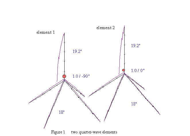
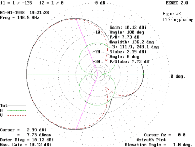
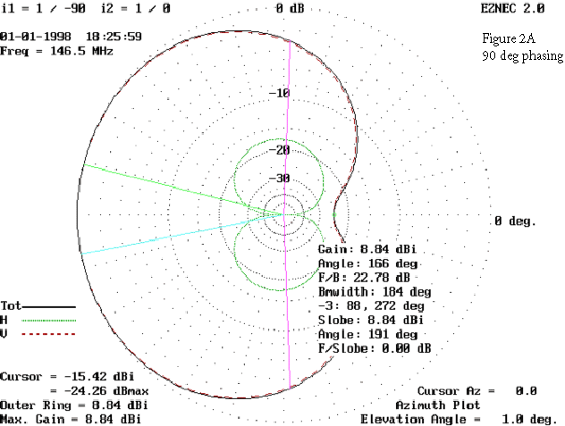 Getting
back to our analysis of the QST construction article1, consider the
case of two quarter-wave elements cut for the two-meter band and spaced a
quarter wavelength, each having four ground radials bent downward at a 45 degree
angle (Figure 1). If the phase of the current in one element is 90 degrees out
of phase with the other, then the fields radiated from these elements are in
phase in one direction, and out of phase in the opposite direction. That is, the
signal reinforces in the beam direction and cancels out back. If the current
magnitudes are equal, the null out back goes to zero. In Figure 1, if the left
element's current phase is -90 degrees relative to the right element's phase,
then by the time the left element's electro-magnetic wave arrives at the right
element a quarter wavelength distant, its overall delay is 180 degrees. So the
signal from the left element cancels that from the right element, and the
pattern develops a null to the right. Just the opposite occurs to the left
bearing (Figure 2A). For other relative phases the pattern may have higher gain,
but a secondary lobe may appear out back, and the front-to-back ratio would be
compromised. Phasing of 135 degrees maximizes forward gain for the given quarter
wavelength spacing (Figure 2B).
Getting
back to our analysis of the QST construction article1, consider the
case of two quarter-wave elements cut for the two-meter band and spaced a
quarter wavelength, each having four ground radials bent downward at a 45 degree
angle (Figure 1). If the phase of the current in one element is 90 degrees out
of phase with the other, then the fields radiated from these elements are in
phase in one direction, and out of phase in the opposite direction. That is, the
signal reinforces in the beam direction and cancels out back. If the current
magnitudes are equal, the null out back goes to zero. In Figure 1, if the left
element's current phase is -90 degrees relative to the right element's phase,
then by the time the left element's electro-magnetic wave arrives at the right
element a quarter wavelength distant, its overall delay is 180 degrees. So the
signal from the left element cancels that from the right element, and the
pattern develops a null to the right. Just the opposite occurs to the left
bearing (Figure 2A). For other relative phases the pattern may have higher gain,
but a secondary lobe may appear out back, and the front-to-back ratio would be
compromised. Phasing of 135 degrees maximizes forward gain for the given quarter
wavelength spacing (Figure 2B).
Physical Particulars
The two vertical antenna elements are 19.2 inches long, and all calculations
in this article were done at 146.5 MHz. The elements are spaced 19.2 inches, and
the image-plane radials are 18 inches long.1 The ground is 30 feet
below the feed-points of the elements. The ground conductivity is 5 mS/m and the
relative dielectric constant is 15. All wire diameters are 1/4 inch. The
transmission lines are lossless RG8, which has a surge impedance of 52 ohms and
a velocity factor of 66 percent. At 146.5 MHz a wavelength in free space is
about 80 inches, but it is only 53 inches in RG8. By convention we assign 360
degrees of phase shift to a wavelength, so a quarter wavelength is 90 degrees. A
piece of RG8 that is physically a quarter wavelength long (in this case, 20
inches) actually has a phase shift of 90/.66 = 136 degrees, but only if the VSWR
is 1.0 (more about this later). The outer conductors of the RG8 were included in
the moment-method antenna model, and formed a vee shape beneath the ground
radials. This affected the pattern only slightly, perhaps 0.2 dB. The gain
figures cited in this article are for an elevation angle of one degree above the
horizon. See appendix for a typical vertical pattern.
 Phase
Shift Sign Conventions
Phase
Shift Sign Conventions
There is some confusion about the sign of the phase shift across a
transmission line -- do we call this 20 inches of RG8 minus 136 degrees or plus
136 degrees? In the commercial broadcast industry most engineers assign a minus
sign to the phase shift across a transmission line, and this is in keeping with
the concept of "delay." That is, the arrival of the RF energy at the end of the
line is delayed by 136 degrees in this case. And if that same energy were
traveling through 20 inches of space, it would only be delayed by 90 degrees. If
we were to model this 20 inch length of transmission line as a tee network, it
would have a capacitor in its shunt leg and identical input and output inductors
in its series arms. If we chose a pi network model, it would have identical
capacitors in the shunt input and output arms, and a coil in the series arm.
I think some of the confusion about the sign convention of phase shift stems
from Circuits 101, where a current entering an inductor is said to lag the
voltage applied to that inductor by 90 degrees, and the current entering a
capacitor is said to lead the voltage across that capacitor by 90 degrees. The
current in the inductor is defined as V/jX, so its phase shift is -90 degrees
relative to the applied voltage, or -jV/X. I suppose it all goes back to the way
we plot waveforms against a time axis. If time increases from left to right on
the graph, then the inductor current sinusoid starts 90 degrees later, which is
to the right of the voltage sinusoid. And in a Cartesian coordinate system we
typically assign positive values to the right of the vertical axis, and negative
values to the left, which tends to contradict the value of -90 degrees we just
defined on the time axis. Again, this is just convention, and if you are
consistent with whatever convention you choose, then your results will be okay.
Above all, remember that we are interested in comparing one current with another
current, not with a voltage.
On the outer ring of a Smith chart is a legend stating which direction is
"towards the generator." When you move in this direction (clockwise) on the
Smith chart, you are moving away from the load, which in the case of our feeder
lines is away from the base of the antenna elements. Keep this in mind, and
everything should work out fine. To check your math, make a rough plot of your
impedance results on the Smith chart to see if everything makes sense. Note that
the phase shift around the complete circumference of a Smith chart is 180
degrees, not 360 degrees.
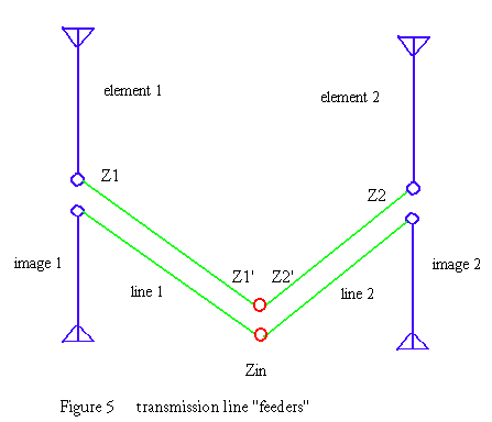
So the practical question becomes, how does one obtain equal current
magnitudes and a relative phase of 90 to 135 degrees in the two antenna
elements? Perhaps the first approach that comes to mind is to feed the two
elements with different lengths of transmission line, one that is a quarter
wavelength longer than the other (Figure 5). However, on closer inspection, this
technique is flawed because it assumes that the transmission lines are
terminated in their characteristic impedance. You see, the current phase shift
through a transmission line is dependent on its load impedance. And the
feed-point "operating" impedances of the two elements in our array are not equal
to each other, nor are they equal to their individual or "self" impedances. This
is caused by the electro-magnetic coupling between the two elements. They are
close enough physically that they influence each other very significantly. So
every time we change the length of one transmission line, the mismatch on
both lines changes, the relative element currents change, etc. In fact,
just about everything interacts in a multi-element antenna. You can't make a
change in one element without influencing the others.
We can get a handle on the amount of coupling and its exact impedance effects
by using the following tee-network model (Figure 3). Think of this as a
transformer model, where the self-inductance of the primary and the secondary
are the same in this case (the two antenna elements are the same), and the
mutual inductance between transformer windings is an analog of the coupling
between the two elements in our array. Except in the world of antennas the
resistance is more significant, so we refer to self and mutual
impedance, rather than inductance. Of course, the mutual impedance
between antenna elements can also be capacitive.
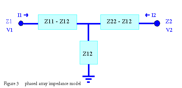
Where Z11 = self impedance of element 1
Z22 = self impedance of element 2
Z12 = mutual impedance between both elements
Z1 = operating input impedance to element 1
Z2 = operating input impedance to element 2
In this case Z11 = Z22, since the array is bilaterally symmetrical
If you prefer, you can model the coupling between elements as a pi network
equivalent (Figure 4) of the tee network we just defined. This might give us
some additional insight into the workings of a phased array. In this case, Z1 =
1/Y1, Z11 = 1/Y11, etc. The port input voltages and currents are the same in
Figures 3 and 4. The pi network has the advantage of having one less "node" than
the tee network, which makes for a more efficient computer analysis model.
Personally I tend to think in series R and X, rather than shunt G and B (even
though those are my initials). Most of us are right-handed, some are
left-handed, and a lucky few are ambidextrous.

Keep in mind that these tee and pi networks are not the same as the standard
impedance matching networks we use in antenna tuners, since those have only one
driven port. Also the impedances seen looking into these antenna models are not
resonant, whereas matching networks typically are. So you can't make too many
safe inferences about antenna behavior based on normal antenna matcher
behavior.
We can measure the self impedance of an antenna element by
connecting our impedance meter to the feed-point of one of the elements when the
other element's feed-point has nothing connected to it. Yes, you must do this in
the presence of the other element, since the self impedance of a single element
alone in free space will not be the same. We can then determine the
mutual impedance by measuring the feed-point impedance when the second
element's feed-point is short-circuited (we will call Z1 in this special case
Zsc), and plugging that value into Equation 1 (does this remind you a bit of the
short-circuit/open-circuit test for measuring transmission line characteristic
impedance?):
_____________
Z12 = sqrt[ Z22 (Z11 - Zsc) ] . . . . . . . . . Equation 1
An alternative approach is to terminate the base of element 2 in an open
circuit, and measure the complex voltage across this termination, V2, and also
measure the complex input current at the base of element 1, I1. Then we could
use Equation 2 to determine the mutual impedance. But since most of us don't
have access to a vector voltmeter, this isn't too practical. However, it is
something we can easily model with a moment-method antenna analysis program.
Z12 = V2 / I1 . . . . . . . . . Equation 2
It should be intuitively obvious that the closer the antenna elements are to
each other, the higher the value of mutual impedance, and the more Zsc will
differ from Z11. If the elements were very far apart, Z12 would be zero and Zsc
would be equal to Z11. Now the real deal is portrayed by the following two
equations, where we can determine what the actual base operating impedances are.
In this case, they are very different from the self-impedances of the two
elements, and the total RF power input to the antenna only rarely splits evenly
between the two elements in a phased array. Remember that the operating
resistance and power of an individual element can be zero, and can also be
negative. However, this is never true at the overall input to the array.
Z1 = Z11 + Z12 (i2/i1) . . . . . . . . . . Equation 3
Z2 = Z22 + Z12 (i1/i2) . . . . . . . . . . Equation 4
Where: i1 = complex base current in element 1
and i2 = complex base current in element 2
The general form of the operating impedance equation for n antenna elements
is
Zi = (Ij/Ii) Zij, for j = 1 to n
Math Example:
The self impedance of these elements is 49.2 + j10.0 ohms, per NEC2 when all
wire diameters are 1/4 inch, and we are 30 feet above 5 mS/m earth. The self
impedance is determined by placing a current source at the feed-point of the
first element, and placing an open-circuit load at the feed-point of the second
element (I used a 10k resistor, which is close enough for our purposes). The
pattern is essentially omni-directional and the gain is 1.4 dBi when the second
element is left "floating" this way. However, it is important to realize that
self-impedance is not determined by de-tuning the other elements in the array in
order to obtain an omni-directional pattern. With electrically taller elements,
say a half wavelength, you may have to short-circuit the parasitic element's
feed-point in order to obtain an omni pattern, and this would yield very wrong
self-impedance values for the driven element. So just ignore the pattern shape
you get when "floating" the other elements in the array. All you care about is
the impedance of the driven element obtained with this test, which we define as
self impedance (Z1 becomes Z11 when there is no current in the output arm of our
Figure 3 tee-network model).
Using Equation 2, the mutual impedance, Z12, is then equal to the voltage
across this 10k resistor, V2, divided by the input current, I1. If you use a
source current of one ampere at zero degrees and NEC to determine what the
current is through the 10k resistor in order to find V2, be careful you don't
get the sign wrong, or your value for Z12 will be off by 180 degrees. This can
occur because in our coupling model of Figure 3, I2 is going into the port, but
in the NEC open-circuit model I2 is coming out of the port. A vector voltmeter
would verify this, but as I said, most of us don't have one. It is always a good
idea to compare your measured or calculated mutual impedance with textbook
values to be sure you haven't made a gross error somewhere.
However, most of us can get our hands on an inexpensive impedance measuring
device, several of which are advertised in the various amateur radio magazines.
When the open circuit at the base of element 2 is replaced with a short circuit,
Z1 = Zsc = 55 + j36.2 ohms. The mutual impedance is then calculated from
equation 1, thus Z12 = 36.7 / -45.6 = 25.7 + j26.2 ohms. By the way, shorting
out the second element makes it act as a reflector, which produces a gain of 4.7
dBi, not bad compared to the 1.4 dBi value we obtained earlier for the
omni-directional pattern.
Now if we drive both elements, we can obtain a maximum gain of 5.2 dBi, which
occurs when the currents are equal in magnitude and phased 135 degrees. If we
phase them 90 degrees, we get a better front-to-back ratio, but less forward
gain (3.9 dBi). So you might ask the question, why should I bother with a
complicated phasing system when I can get pretty good gain simply by feeding one
element and tuning the other as a parasitic reflector? This is a good point, but
if you want the sharpest possible null out the back, you can't do it unless you
independently control the phase and magnitude of the currents. And when the QRM
originates from the back lobe of your antenna's pattern, you might wish for a
better front-to-back ratio, regardless of forward gain. A second and perhaps
more important reason for having a simple method to adjust the relative current
magnitudes and phases is to compensate for stray capacitance and inductance
within the feeder system and the antenna, undesired radiation from the feeder
lines, construction irregularities, etc.
Table 1 describes the differences for various element currents when 100 watts
of power is delivered to the array. Note that dBi is the maximum gain of the
pattern relative to an isotropic radiator, and dBf is the front-to-back ratio of
the pattern. The parasitic case looks attractive (where the second element is
not driven and has no insulator between it and its counterpoise radials). How
can we tell when an element is parasitic? Answer: when it has current but no
power (i.e., when its operating resistance is zero, or it is
short-circuited).
Table 1 Effects of Adjusting Element Currents
input impedance at bases complex current at bases (watts)
gain
Z1 (ohms). . . Z2 (ohms) . . . i1 (amps) i2 (amps) . . . P1 P2 . . . dBi
dBf
75.5 + j35.7 23.1 - j15.8 . . . 1.00 / -90 1.00 / 0 . . . . 77 23 . . . 8.8
22.8
49.6 + j46.7 12.5 + j10.3 . . 1.27 / -135 1.27 / 0 . . . . 80 20 . . . 10.1
7.7
55.1 + j36.2 0.0 + j0.0 . . . . 1.35 / -123 0.98 / 0 . . . 100 0 . . . . 9.6
8.7
53.0 + j26.8 -27.5 - j5.7 . . . 1.46 / -123 0.69 / 0 . . . 113 -13 . . . 8.9
5.6
Negative Resistance
You might be wondering if it is possible to create a situation where one of
the operating resistances is actually negative. In this case the power in one
element would be negative, and the power in the other element would actually be
greater than the total input power to the antenna. This may sound strange, but
it does happen in practice. The sum of all the element powers must equal the
total input power to the antenna. The negative element is passing power back
down its transmission line, and the positive element is passing some of its
power to the negative element. To see it in our simple array, all we have to do
is change the relative current. We know that the parasitic case has zero
resistance at the base of the reflector, so we can start from there by reducing
the magnitude of the element 2 current while maintaining the same phase relative
to element 1. The pattern obtained with this particular negative resistance case
isn't that great, and the bandwidth is likely to be narrower compared to a
comparable pattern obtained from an array having all positive operating
resistances. The negative resistance implies an increased circulating current.
But there are some instances where a very sharp null is desired in the pattern,
and a negative resistance element is the only way to get it. The correct method
of returning the negative power to the common feed-point in phase is widely
misunderstood, but is not something we need to discuss in detail at this
time.3
Feed Lines
So how can we feed this array with the desired complex currents (i1 = 1.0 /
-90 and i2 = 1.0 / 0)? Let's start with a pair of transmission lines per Figure
5, and look at two cases. In both cases we connect 23 inches of RG8 to element
1. In the first case line 2 (connected to element 2) is 17 inches long, but in
the second case it is 3 inches long. In both cases the RF current takes longer
to get from the common feed point of the two transmission lines to element 1
than it takes to get to element 2. We would expect the relative phase in the
first case to be less than it is in the second case, since the difference in
physical line lengths is 6 inches in the first case and 20 inches in the second.
A wavelength at 146.5 MHz in RG8 is 53 inches, so the phase difference in the
first case is (6 / 53) 360 = 41 degrees if the VSWR is 1.0, and in the second
case it is 135 degrees. In practice, the actual phase shifts turn out to be much
different because the lines are not matched. In fact the relative phase in the
first case is 91 degrees, and in the second case is 150 degrees. So we missed
the boat by 50 degrees in the first case, and by 15 degrees in the second case
(Table 2). But since we actually wanted a relative phase of 90 degrees, rather
than 41 degrees, our first case looks pretty good as a practical feeder
solution. When I say relative phase I mean that i2 leads i1 by 90 degrees, or i1
lags i2 by 90 degrees.
Table 2 Effects of Feeding with Mis-matched Lines
input impedance at bases . . . . . current at bases . . . . . power
(watts)
case Z1 (ohms) Z2 (ohms) . . . i1 (amps) i2 (amps) . . . P1 P2 . . . . .
dBi dBf
1 73.0 + j41.4 30.4 - j18.3 . . . 0.91 / -91 1.11 / 0 . . .
61W 39W . . . 9.2 22.3
2 32.1 + j41.7 15.6 + j8.8 . . . 1.40 / -150 1.54 / 0 . . .
63W 37W . . . 10.9 5.5
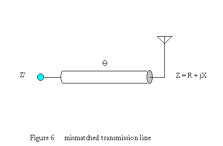 Keep in
mind that the sign of the electrical length of the transmission line is normally
construed as positive, but the current phase shift is normally considered
negative to connote the time lag associated with travel through the line. So in
Figure 6, if we have a quarter wavelength line, we say that theta is 90 degrees.
However, the phase shift phi associated with this line is - 90 degrees, for the
matched condition. The formulas listed in this article assume that the value for
theta is positive. So think electrical length when you see theta, and think
time-lag phase shift when you see phi.
Keep in
mind that the sign of the electrical length of the transmission line is normally
construed as positive, but the current phase shift is normally considered
negative to connote the time lag associated with travel through the line. So in
Figure 6, if we have a quarter wavelength line, we say that theta is 90 degrees.
However, the phase shift phi associated with this line is - 90 degrees, for the
matched condition. The formulas listed in this article assume that the value for
theta is positive. So think electrical length when you see theta, and think
time-lag phase shift when you see phi.
The transmission lines are terminated in the impedances above, so they are
mismatched. The lines transform their load impedances (Equation 5) to the Z1'
and Z2' values in Table 3 below. The combined input impedance Zin at their
common junction is simply Z1' in parallel with Z2'. The current phase shift
through the mismatched transmission lines can be determined with Equation 6. If
we change the line lengths in an attempt to produce higher gain, comparing case
2 to case 1 above our impedance match becomes even worse, as the element
currents increase and the operating resistances decrease farther below the 52
ohm characteristic impedance of the transmission line. Increased currents for a
given power is the price you pay for higher gain.
We don't have to use a moment-method antenna analysis program to determine
the currents in the individual array elements. Instead we can simply plug into
an AC network analysis program the tee network model of the coupled antenna
elements per Figure 3, and the two feeder lines. If the network analysis program
does not have a transmission line model, you can make your own pi or tee network
equivalent.
Table 3 Mis-matched Feeder Lines
. . . . . . . Input 1. . . . . . . . . . . . . . . . . . . . Input 2 . . . .
. . . . . . . . . . . . . .Combined
line1 . . Z1' (ohms) . . VSWR . . . . line 2 . . Z2' (ohms) . . VSWR . . .
. Zin (ohms) . . VSWR
23 in 39 + j31 ohms . . 2.08 . . . . . 17 in . 104 + j4 ohms . . 2.00 . . . .
. 31.6 + j15.2 . . 1.85
23 in 20 + j18 ohms . . 2.96 . . . . . . 3 in . 108 + j6 ohms . . 2.09 . . .
. . .18.5 + j12.7 . . 3.00
Z' = (Z - jZo tan Theta) / (1 - j [Z / Zo] tan Theta) . . . . . . . . . . .
Equation 5
Phi = tan-1 [ R / (X + Zo / tan Theta)] . . . . . . . . . . . . . .Equation
6
Note that the current phase shift through the transmission lines given by
Equation 5 is only part of the story. There is an additional phase shift that
occurs at the common end of the transmission lines because the input current
does not split evenly between the two lines. That is, the input impedance to
each line is different (Z1' and Z2'). Finding this additional phase shift
requires a simple exercise of Ohm's Law, where the relative phase of the two
input currents can be determined by Equation 7.
i2' / i1' = Z1' / Z2' . . . . . . . . Equation 7
So what we have done by decreasing the length of line 2 is to compromise our
impedance match in order to obtain maximum gain, but in neither case do we have
a sharp null out the back because the element current magnitudes are never
equal. Is there some other combination of transmission line lengths and types
that would offer a better impedance match and also produce the desired pattern?
Maybe, but finding it could be a painfully iterative process. It is not
something you would want to do while standing on a ladder, that's for sure (does
this sound familiar?).
Practical Adjustment Techniques
Before we get into a full-blown phasing and coupling network design, let's
look at what a single variable capacitor installed at the input to element 1
buys us in the way of adjustability. We know from Table 1 that the inductive
input reactance to this element varies from 27 to 47 ohms for the range of
radiation patterns that interest us. If we tune this out with a capacitive
reactance, we reduce the VSWR on line 1 and we also afford some adjustability of
the pattern (Table 4). However, the pattern degrades with a capacitor, but gives
us what we want with an inductor. So intuition doesn't always work in a
mis-matched feed system, does it? Apparently the design is relying heavily on
mismatch to produce additional phase shift in the transmission line. The
following is for the case where we have 23 inches of RG8 connected to element 1
and 17 inches of RG8 connected to element 2. Note how touchy the pattern is;
this should tell you to be very careful with your transmission line wiring
because even a little inductance has a big effect at the base of the driven
elements. It should also tell you that you need a practical adjustment handle if
you want the pattern to arrive when and where you expect it. Take a while to
appreciate the range of forward gain and front-to-back values in Table 4 that
can be had with a simple turn of a variable capacitor in series with a fixed
inductor.
Table 4 Pattern Adjustment with Series Coil and Capacitor at Element
1
#1 tuning. . . . . . . . . . . . . . current at bases
reactance . . . Zin (ohms) . . . . i1 (amps) i2 (amps) . . dBi dBf
-30 ohms . . 35 + j11 ohms . . 0.62 / -56 1.10 / 0 . . . . 7.9 4.5
-20 ohms . . 34 + j12 ohms . . 0.65 / -65 1.08 / 0 . . . . 8.2 6.7
-10 ohms . . 33 + j13 ohms . . 0.80 / -76 1.08 / 0 . . . . 8.6 10.9
0 ohms . . . .32 + j15 ohms . . 0.91 / -91 1.11 / 0 . . . . 9.2 22.3
10 ohms . . . 31 + j18 ohms . . 1.02 / -107 1.21 / 0 . . . 9.9 19.6
20 ohms . . . 31 + j21 ohms . . 1.08 / -123 1.36 / 0 . . 10.4 12.0
30 ohms . . . 33 + j25 ohms . . 1.08 / -137 1.53 / 0 . . 10.6 8.1
40 ohms . . . 36 + j27 ohms . . 1.02 / -146 1.65 / 0 . . 10.4 5.7
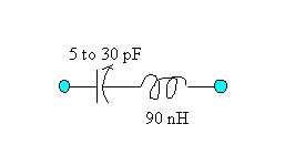 Intuition
suggests that if an inductor in series with element 1 gives us the adjustment
range we want, then perhaps a capacitor in series with element 2 would do the
same. A small variable capacitor seems better suited to our application than a
variable inductor, so to cover the reactance range of -40 to +40 ohms we could
use a variable capacitor in series with a fixed coil. In the 2 meter band, a 5
to 30 pF variable capacitor in series with a 90 nH air-core coil would work fine
(about three turns on a half inch diameter).
Intuition
suggests that if an inductor in series with element 1 gives us the adjustment
range we want, then perhaps a capacitor in series with element 2 would do the
same. A small variable capacitor seems better suited to our application than a
variable inductor, so to cover the reactance range of -40 to +40 ohms we could
use a variable capacitor in series with a fixed coil. In the 2 meter band, a 5
to 30 pF variable capacitor in series with a 90 nH air-core coil would work fine
(about three turns on a half inch diameter).
Table 5 tells the story of what happens when we tune the base of element 2,
and it should be no surprise that again the results are not as expected.
Specifically we just don't get the big forward gain that we get by tuning at the
base of element 1. So it looks like we have to use an inductive reactance in
series with element 1 in order to get the maximum gain from our array. Perhaps
adjustment at the base of element 2 is less effective because there is less
power in this element?
Perhaps a variable capacitor at the input to one of the transmission lines
will do the trick. Or perhaps a variable capacitor at the input and output of
both transmission lines would give us enough adjustment latitude. Or would it
just serve to get us lost in the woods? I leave this as an exercise for the
reader, because I don't believe in taking all the fun out of a project and
leaving no room for experimentation. Remember that at these relatively low power
levels, using mis-matched feeder lines is not a bad practice, so take advantage
of it.
Table 5 Pattern Adjustment with Series Coil and Capacitor at Element
2
#2 tuning . . . . . . . . . . . . . current at bases
reactance Zin (ohms) . . . i1 (amps) i2 (amps) . . . dBi dBf
-40 ohms 24 + j22 . . . . . 1.02 / -85 0.84 / 0 . . . . . 8.9 13.2
-30 ohms 26 + j21 . . . . . 1.08 / -86 0.90 / 0 . . . . . 9.0 15.6
-20 ohms 28 + j20 . . . . . 1.04 / -87 0.96 / 0 . . . . . 9.0 19.1
-10 ohms 30 + j18 . . . . . 0.98 / -89 1.03 / 0 . . . . . 9.1 23.4
0 ohms 32 + j15 . . . . . . . 0.91 / -91 1.11 / 0 . . . . . 9.2 22.3
10 ohms 33 + j11 . . . . . . 0.83 / -87 1.20 / 0 . . . . . 9.2 16.9
20 ohms 32 + j6 . . . . . . . 0.73 / -98 1.29 / 0 . . . . . 9.2 12.6
30 ohms 30 + j1 . . . . . . . 0.62 / -111 1.38 / 0 . . . . 9.1 9.3
There is nothing egregiously wrong with having a high VSWR on the feeder
lines. The extra losses and higher voltages and currents in short feeder lines
caused by the mismatch are not too significant at ham radio power levels, in
most cases. But remember, the higher the gain, the higher the currents in those
feeder lines. If you are in doubt, be sure to calculate all component voltages
and currents, and be aware that the wet voltage ratings at the ends of the lines
are a lot lower than the ideal dry sea-level ratings (yes, you have to de-rate
for altitude).
Of course, some effort should be made to match the main transmission line at
the common junction of the feeder lines, since the main line is a lot longer
than the feeders and its overall power loss could be significantly higher in the
mis-matched condition. A couple of stubs would do the trick, as long as we are
careful that they don't become additional parasitic radiating elements in our
array.
The alternative to the mis-matched feeder approach is to match the operating
base impedance of each element to the transmission line surge impedance, and to
provide a controlled-phase-shift power divider at the common input to the array.
But we need to keep track of the phase shift across the element matching
networks, too. And it is not that easy to make an impedance matching network
that works well in the two-meter band, and has independent phase and impedance
transformation adjustability. We could make a tee network phasing and coupling
unit out of three stubs. A quarter wavelength ladder-line stub with a sliding
short would work well as an inductor, and an adjustable length open-circuited
stub would work as a capacitor, but then you have to deal with the problem of
parasitic re-radiation from the stubs. That is, the stubs start to act as
undesired antenna elements. So a lumped parameter tee network may be the best
approach, since these components would be considerably smaller than the stubs.
An adjustable co-axial capacitor is easy to fashion from a couple inches of
half-inch copper pipe stuffed with a plastic dowel bored and tapped to accept a
3/8 inch diameter screw. This gives you a surge impedance of about 10 ohms,
which yields about 14 pF per inch. A 5/16 inch screw would yield about 9 pF per
inch, and a 1/4-20 screw about 6 pF per inch. A DC capacitance meter will get
you in the ball park, but it is safer to use an impedance meter at VHF, if you
use it properly. The time-honored method of playing an air-core solenoidal coil
like an accordion provides a practical form of adjustable inductor. Or you could
try an adjustable ferrite slug, if you can find one that is not too lossy at 146
MHz. In any case you need to make a good estimate of the initial component
values, which means you need to utilize the formulas and measurement techniques
in this article or run a moment-method analysis to determine what your
driving-point impedances are likely to be.
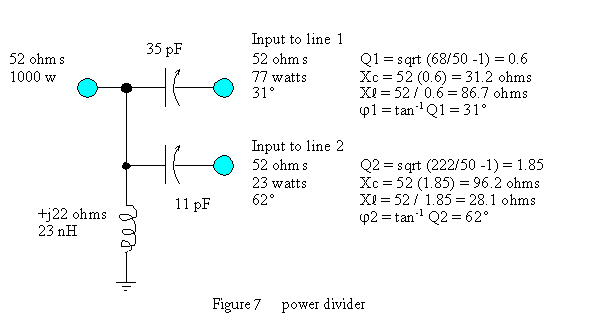
Phasing and Coupling Network Example
Assume we really want equal current magnitudes in each element, and a
relative phase of 90 degrees. We already know the driving point impedances and
powers to expect. Now we want to match those impedances to 52 ohms, and we also
want 52 ohms at the common feed point to the array. Let's start at the power
divider, using what is called an Ohm's Law configuration. We know that element 1
radiates 77 watts and element 2 radiates 23 watts. In order for more power to be
transferred to line 1, we need to present a lower resistance to the common input
point looking towards line 1 as compared to line 2 (V2/R). We also
know that the paralleled resistances looking toward the two lines is 52 ohms. So
for 100 watts input to the array the math looks like this, where V is the input
voltage across the power divider:
V2 = PR = 100 (52) = 5200
V2 / R1 = 77 watts, so R1 = 68 ohms
V2 / R2 = 23 watts, so R2 = 222 ohms
Checking our work, R1R2 / (R1 + R2) = 52 ohms
So if we connect an L network between the common point and each transmission
line, we might have a network that looks like Figure 7. Note that the shunt
elements of the two high-pass L networks combine to form one coil. I chose
"leading" phase shift networks, as opposed to "lagging" phase shift, low-pass
networks simply because it is cleaner and easier to adjust a co-axial screw
capacitor than it is to adjust a coil. So I end up with two capacitors and one
coil, instead of two coils and one capacitor. A co-axial screw inductor would be
physically too long for this application, in my opinion, because it would begin
to act as another radiating element in the array. However, if you are willing to
add more-or-less a quarter wavelength of line to your capacitor, you can make it
look like an inductor. Note that the two capacitors in the power divider are not
connected to ground, so you have to be careful how you mount them. If you make
them from ½ inch copper pipe, you could align the pipes in parallel and solder
them together, and this would form the common side of the power divider.
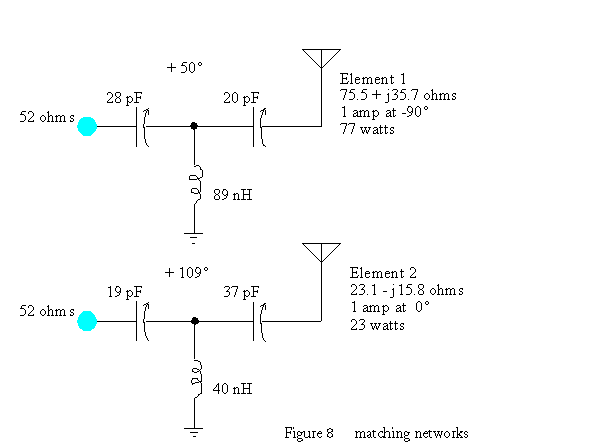
Now that we have taken care of the front end of our phasing and coupling
design, we need to determine the phase shift needed in the impedance matching
units at the other ends of the feeders. Note that the phase shift across the two
legs of the power divider are not equal -- leg 1 lags 31 degrees behind leg 2
(62 - 31 = 31). In order to simplify our design, let's use equal length feeder
lines. This has the benefit of creating a symmetrical perturbation of the
antenna structure and will tend to minimize pattern distortion and other
side-effects. We want the relative current in element 1 to lag that of element 2
by 90 degrees. We already have 31 degrees of lag provided by the power divider,
so we need an additional -59 degrees. We can get this by selecting a phase shift
across matching network 1 of 50 degrees, and across matching network 2 of 109
degrees per Figure 8. The component values shown are for 146.5 MHz.
During adjustment it may also be useful to have a dual-trace, wide-band
oscilloscope to monitor the currents and phases in each element using a small
sample loop located near, but not connected to, each element. However, you would
have to be very careful with the placement and de-tuning of your sample lines so
as not to disturb the array. This gets complicated at VHF. Unless you are very
patient, this may be more trouble than it is worth. However, it is quite
practical at lower frequencies.
It would be nice to have two helpers with hand-held 2-meter transceivers, one
aligned with the main bang of the antenna, and the other on the other side. Then
you could communicate with them using your transceiver plugged into the antenna
under test. As you adjusted your phasing and coupling components, your helpers
would relay their S-meter readings back to you. Or you could use a single
helper, and rotate the antenna 180 degrees of azimuth to measure the forward and
reverse fields. Be sure to maintain a constant input power to the antenna when
you do this; an auto-tuner would be ideal for these circumstances. If you don't
have a helper, you could key down the hand-held and leave it radiating in your
neighbor's pasture while you adjust your antenna for maximum received signal in
the forward direction, and minimum signal in the reverse direction. Keep a
clip-board and pencil at your side to keep track of component settings and the
resulting field intensities. Otherwise you may lose your bearings and end up
repeating the same tests.
Summary
In summary, the technique of connecting mismatched feeders to the driven
elements in a phased array is an expedient method for obtaining relative current
phases that approximate the desired values. A variable capacitor in series with
one or more of the lines will often provide a good degree of adjustability.
However, it won't always work, in which case phasing and coupling networks may
have to be inserted between the elements and the feeder lines, and a power
divider will have to be constructed at the input to the feeders. In order for
this approach to be successful, it implies a knowledge of the operating feed
impedances of the driven elements, and the way they interact with one another.
In actual practice it can be a real "can of worms." A simplified approach that
will allow easy adjustability of the pattern is therefor suggested where a
single series coil and/or capacitor is inserted at the feed-point of one or more
of the driven elements. In all cases where lumped parameters are added to the
design, impedance and pattern bandwidth may suffer, but this needs to be
addressed on a case-by-case basis. If your moment-method program does not allow
you to enter all the network components in your phasing and coupling equipment,
a network analysis program can do the job if you model the antenna self and
mutual impedances using the multi-port network models discussed in this
article.
You don't need an antenna analysis program to measure and model the
interaction between radiating elements in an antenna; all you need is an
impedance measuring device, some math skills, and some network analysis
software. However, a moment-method program is certainly helpful, and should be
part of your arsenal of design tools. Sometimes the stray reactances and pattern
"scattering" within and around an antenna can mask what is really going on, and
if you can approach an antenna problem simultaneously from different angles, you
will converge on a design solution in less time.
A note about the mutual coupling model -- I used a tee network in this
article, but a special pi network requiring some fancy matrix math is the
practical form when more than two antenna elements are used.2
Topologically a pi network has one less voltage node than a tee network, and
this has advantages over a tee network. However a detailed discussion of the
generalized antenna impedance model is beyond the scope of this article, so I
have attached an appendix giving just the basics.
References:
1) Harold Thomas, "A 2-Meter Phased-Array Antenna," January 1998,
QST.
2) Dane Jubera, "Toward Improved Control of Medium Wave Directional Arrays,"
December 1981, IEEE Transactions on Broadcasting.
3) Grant Bingeman, "Negative Towers," November 1980, Broadcast
Management/Engineering.
____________________________________________________________________
author's biography:
Grant Bingeman, P.E., KM5KG (ex-WN6AIW, WB6MBX, WB4AOI) has been a Senior
Engineer at Continental Electronics in Dallas, Texas for 17 years, where he
designs high power antennas and transmitters. Call him at 214-381-7161 and he'll
give you a special deal on a 500 kw auto-tuned short-wave transmitter. His
e-mail address is DrBingo@compuserve.com.
______________________________________________________________________
Appendix
A rigorous multi-port network model of a phased
array containing n radiating elements can be developed using the following
procedure. First form a matrix of the mutual impedances between all the
elements. This matrix will contain n2 complex values, and look like
this:
Z11 Z12 ... Z1n
Z21 Z22 ... Z2n
. . .
. . .
Zn1 Zn2 ... Znn
Then you
must invert the matrix, keeping in mind that matrix inversion is a tedious math
process that you will probably not want to program yourself, but simply call as
a function from a math library. In other words, an individual matrix element Yij
does not equal 1/Zij.
Y11 Y12 ... Y1n
Y21 Y22 ... Y2n
. . .
. . .
Yn1 Yn2 ... Ynn
Next you must calculate the lumped-parameter
values for the network shown in Figure 9, using these equations:
Zi' = 1 / [Yi1 + Yi2 + ... + Yin]
Zij' = -1 / Yij
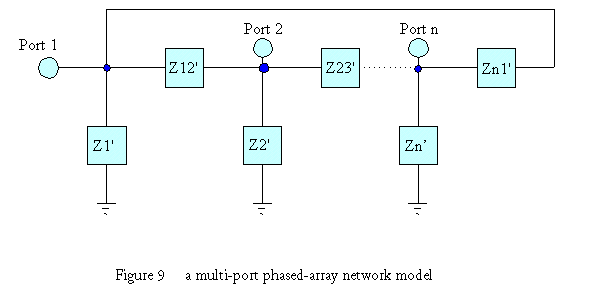
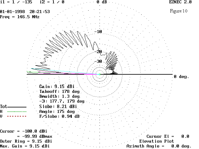
Figure 10 shows the vertical or elevation
pattern of the array described in Figure 1 when the element currents are equal
in magnitude and phased 135 degrees. The forward gains and front-to-back ratios
will vary depending on the elevation angle of interest. The values throughout
this article are for an elevation angle of one degree above the horizon plane.
Since communication at these frequencies is almost always line-of-sight, this is
a valid angle. Note that the far-field goes to zero when the elevation angle is
zero, but the near field does not. For 100 watts input to the array, you can
expect a vertically polarized field intensity at one kilometer two meters above
ground of about 1.5 mV/m for the pattern shown in Figure 10 on a bearing of 270
degrees true over 5 mS/m earth, assuming no reflections. This value would be
slightly higher if the ground conductivity were better. Over perfect ground the
field would be about 12 mV/m.
file: array.wpd 3-10-98